
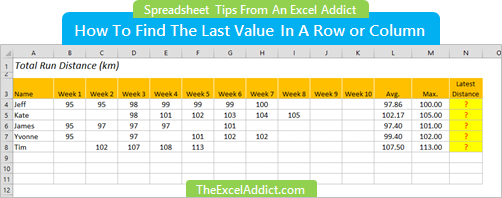
How To Find The Last Value In A Row or Column
by Francis Hayes (The Excel Addict)
When you want to do a seemingly common spreadsheet task and cannot find a solution, it can often be both frustrating and astounding that the folks at Microsoft hadn't thought of including that functionality. One example of this is the need to return the last value in a row or column.

As with many Excel challenges, there are often multiple possible solutions available. So, whenever I need to find the last value in a row or column, I use this interesting solution that uses a combination of Excel's INDEX and MATCH functions.
To find the last numeric value in a row that may also include blank cells, try this formula;
=INDEX(row_lookup_range,MATCH(9.99999999999999E+307,row_lookup_range))

=INDEX(B4:K4,MATCH(9.99999999999999E+307,B4:K4))
The row_lookup_range is the range of cells (B4:K4) in a single row or an entire row (2:2) in which we want to find the last numeric value. The interesting thing about this formula is the way it uses the MATCH function.
MATCH(lookup_value,
lookup_range,
match_type)
If you are familiar with Excel's lookup functions, you will know that they can be used to find an exact match or a closest match. In the MATCH function, this is determined by the third argument of the function (i.e. match_type), which by default, if omitted from the formula is 1 (or the closest match), and finds the largest value in the lookup_range that is less than or equal to the lookup_value.
In most cases with the MATCH function, the values in the lookup range are required to be in ascending order. However, in this case, we don't need to have the values in ascending order, so we can use this to help solve our problem.
Explanation of the MATCH(9.99999999999999E+307,row_lookup_range) part of the formula:
This part is actually pretty simple and a little clever. Here, for the lookup_value we will use the highest possible numeric value in Excel (i.e. 9.99999999999999E+307) so that it will be higher than any possible value in our row_lookup_range. In fact, you could use 1,000,000 for the lookup value if you know the maximum value in the row_lookup_range will always be less than a million.
When the MATCH function looks through the row_lookup_range from left to right for the lookup_value, it doesn't find it. Since the match_type argument of the function is omitted, by default it looks backward from the rightmost cell in the range and returns the last numeric value that is less than or equal to the lookup_value (i.e. 9.99999999999999E+307). This turns out to be the last numeric value in the row_lookup_range.
To find the last NUMERIC value in a COLUMN...
...we
can adapt the same formula by supplying a column_lookup_range.
=INDEX(A1:A500,MATCH(9.99999999999999E+307,A1:A500))
To find the last TEXT value in a ROW...
...we
use the REPT function to create a lookup_value
that is string of Zs 255 characters long so that,
alphabetically, it will be larger than any text
found in the row.
=INDEX(B1:W1,MATCH(REPT("Z",255),B1:W1))
To find the last TEXT value in a COLUMN...
...we
simply replace the row_lookup_range
with a column_lookup_range.
=INDEX(A1:A500,MATCH(REPT("Z",255),A1:A500))
If your lookup range does not include blanks...
...you
can use a simpler approach with these formulas...
For
Rows: =INDEX(B1:W1,COUNTA(B1:W1),1)
For
Columns: =INDEX(A1:A500,COUNTA(A1:A500),1)
If your formula returns #N/A:
If any of these formulas result in a #N/A error because there is no numeric value when using the numeric formula or text value when using the text formula, you can modify your formula with an IFERROR function to return a blank instead of an error:
=IFERROR(INDEX(B4:K4,MATCH(9.99999999999999E+307,B4:K4)),"")
or
=IFERROR(INDEX(B1:W1,MATCH(REPT("Z",255),B1:W1)),"")
Do you use a different method for Finding The Last Value In A Row or Column? Please tell me about it.
If you found this tip helpful, please share it with your Excel friends and colleagues.
To get more tips every week like this one...
'Spreadsheet Tips From An Excel Addict'
'Excel in Seconds' & 'Excel in Minutes'
Plus you also get my 'Excel in Seconds' E-book as a BONUS!
(Download it immediately after you sign up)
Copyright Francis Hayes © All Rights Reserved
8 Lexington Place, Conception Bay South, NL Canada A1X 6A2
Phone 709-834-4630
This site is not affiliated with Microsoft Corporation.