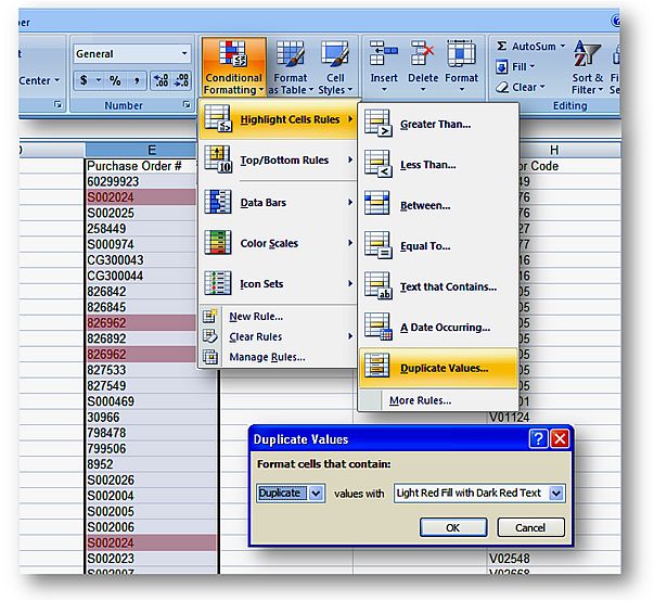
In previous versions of Excel , it took a multi-step approach using a COUNTIF formula in Conditional Formatting to highlight duplicate values in your data. Beginning with Excel 2007, highlighting Duplicate Values got a whole lot easier.
You simply click Conditional Formatting on the Home tab, then point to Highlight Cell Rules, Duplicate Values and click OK.

If you'd prefer to highlight your cells with a different color, you can do that too or you can choose a completely different formatting (e.g. red + bold + strikethrough) by clicking the Custom... option at the bottom of the dropdown menu and choosing your formatting.
The great thing about using Conditional Formatting to highlight duplicates is that this is not just for a one-time highlighting of duplicate values. Doing this applies Conditional Formatting to the range of cells you select so that in the future, when more data is added, any duplicates will be automatically highlighted.
Note however that with a normal range of cells, this Conditional Formatting will be applied only to the range you select. If additional records are subsequently added to your data, they will not have the Conditional formatting applied to them. The best way to avoid this to format the range as an Excel table. From the Home tab, choose Format as Table. With an Excel table, as more data is added to the table, the formatting will be copied down from the cells above.
|
Would you believe me if I told
you that
you can DOUBLE your productivity in Excel? How about TRIPLE it ? or QUADRUPLE it ? or MORE ? If I showed you a tip where you could do a task in Excel in five seconds that would typically take you 20 minutes to an hour or more, what would you call that? Productivity on steroids? ...and that's just ONE tip! "Give me 10 or 15 minutes each week and I will show you how learning a few of my time-saving 'Spreadsheet Tips From An Excel Addict' on a regular basis will seem almost effortless BUT will quickly help you BOOST your productivity in Excel beyond your imagination" Francis Hayes, The Excel Addict Get my FREE Twice-Weekly
Newsletter
"Spreadsheet Tips From An Excel Addict" Now being read by more than 37,000+ Excel Addicts all over the world |
Microsoft and the Microsoft Office logo are trademarks or registered trademarks of Microsoft Corporation in the United States and/or other countries. Product names, logos, brands, and other trademarks featured or referred to within this website are the property of their respective trademark holders.